A Brief Introduction to Machine Learning for Engineers 2 Part II
2. A “Gentle” Introduction Through Linear Regression
2.3 Frequentist framework:
Maximum a posteriori (MAP) learning
Model order \(M\) dictates the trade off between low bias (high \(M\)) and low estimation error (low \(M\)). MAP approach enables refined control over 2 metrcis by assigning a distribution to model parameters.
For instance observing high capacity model (larger \(M\)) leads to bigger value model parameters (\(w\)). We can use this information to limit or distribution to \(w\).
\[w \sim \mathcal{N}(0, \alpha^{-1}I), ~~ \alpha \text{ is precision}\]Rather than maximizing likelihood \(P(t_{D} \vert X_{D}, w, \beta)\), we maximize the posteriror distribution:
\[P(t_{D}, w \vert X_{D}, \beta) = P(w) \prod_{j=1}^{N} P(t_{j} \vert x_{j}; w, \beta)\]Following the same line of argument in maximum likelihood, negative \(\ln\) of posterior probability is
\[- \ln P(t_{D}, w \vert X_{D}, \beta) = - \ln \left(\prod_{j=1}^{N} P(t_{j} \vert x_{j}; w, \beta) \right) - \ln(P(w))\] \[= - \ln ~ \left( (\frac{\beta}{\sqrt{2\pi}})^{N} \exp \left(-\frac{1}{2} \frac{\sum_{n=1}^{N}~(t_{n} - \hat{t})^{2}}{\beta^{-1}} \right) \right) - \ln \left( \frac{1}{\sqrt{2\pi} \sqrt{ \vert \alpha^{-1}I} \vert }) \exp \left(-\frac{1}{2} w^{T} (\alpha^{-1} I)^{-1} w \right) \right)\]First term is the same as in maximum likelihood, so we already know that
\[= - \frac{N}{2} \ln(~ \frac{\beta}{2\pi}~ ) +\frac{\beta}{2} \sum_{n=1}^{N}~(t_{n} - \hat{t}(x_{n})^{2} - \frac{1}{2} \ln(~ \frac{\alpha^{M}}{2\pi}~) + \frac{\alpha}{2} \vert \vert w \vert \vert ^{2}\]and let’s unpack derivations in the second term, since w is in fact a multivariate distribution we have to use covariance matrix \(\alpha^{-1} I\), nevertheless since it is a diagonal matrix, determinant of it is just the product of its diagonal elements which are equal to \(\alpha^{-1}\). In addition, \(w^{T} (\alpha^{-1} I)^{-1} w = \alpha w^{T} w = \alpha \vert \vert w \vert \vert ^{2}\) again due to covariance being diagonal with the same \(\alpha^{-1}\) elements.
Finally, disregarding constant terms and dividing the expression by \(\beta N / 2\) we get
\[- \ln P(t_{D}, w \vert X_{D}, \beta) = \underset{w}{min} ~ \mathcal{L_{D}}~(w) + \frac{\lambda}{N} \vert \vert w \vert \vert ^{2}, ~~~~ (2.27)\]where \(\lambda = \alpha / \beta\) is called regularization constant. An important observation is that when N grows significantly, problem transforms int maximum likelihood. Using the same steps in maximum likelihood, we can also solve this minimization problem analytically.
\[= \frac{1}{N} \vert \vert t_{D} - X_{D}~w \vert \vert ^{2} + \frac{\lambda}{N} \vert \vert w \vert \vert ^{2}= \frac{1}{N} (t_{D} - X_{D}~w)^{T} (t_{D} - X_{D}~w) + \frac{1}{N} w^{T} \lambda I w\] \[= \frac{1}{N}~(t_{D}^{T}~t_{D} - t_{D}^{T}~X_{D}~w - w^{T}~X_{D}^{T}~t_{D} + w^{T}~X_{D}^{T}~X_{D}~ w) + \frac{1}{N} w^{T} \lambda I w\] \[= \frac{1}{N}~(t_{D}^{T}~t_{D} - \underset{\text{scalar so transpose is the same}}{(t_{D}^{T}~X_{D}~w)^{T}} - w^{T}~X_{D}^{T}~t_{D} + w^{T}~X_{D}^{T}~X_{D}~ w) + \frac{1}{N} w^{T} \lambda I w\] \[= \frac{1}{N}~[(t_{D}^{T}~t_{D} - 2w^{T}~X_{D}^{T}~t_{D} + w^{T}(X_{D}^{T}~X_{D}~ w)] + \frac{1}{N} w^{T} \lambda I w\]Since our starting expression is convex and has a global extremum, if we take the derivative of the expression above with respect to w and set it to 0:
\[\frac{\partial \mathcal{L_{D}}~(w) + \frac{\lambda}{N} \vert \vert w \vert \vert ^{2}}{\partial w} =\frac{1}{N}[ 0 - 2 X_{D}^{T}~t_{D} + (X_{D}^{T}~X_{D} + (X_{D}^{T}~X_{D})^{T})~w + \frac{ 2\lambda I }{N}~w] = 0\] \[\text{Since } X_{D}^{T}~X_{D} \text{ is symmetric } =\frac{1}{N} [0 - 2 X_{D}^{T}~t_{D} + 2 X_{D}^{T}~X_{D}~w + \frac{ 2\lambda I }{N}~w] = 0\] \[X_{D}^{T}~X_{D}~w + \lambda I w = X_{D}^{T}~t_{D}\] \[(X_{D}^{T}~X_{D} + \lambda I) w = X_{D}^{T}~t_{D}\] \[(\lambda I + X_{D}^{T}~X_{D})^{-1} (\lambda I + X_{D}^{T}~X_{D})~w = (\lambda I + X_{D}^{T}~X_{D})^{-1} X_{D}^{T}~t_{D}\] \[w_{MAP} = (\lambda I + X_{D}^{T}~X_{D})^{-1} X_{D}^{T}~t_{D}\]Regularization
Regularization is used to prevent overfitting and find the optimum model capacity meaning model order M. In previous explanation, it is shown that MAP amounts to ML or ERM with regularization. Furthermore, we can introduce \(R(w)\) to ML or ERM independent of probabilistic interpretation. For example we can inspect our training results and conclude that higher \(w\) values induce overfitting and use \(R(w) = \frac{\lambda}{N} \vert \vert w \vert \vert ^{2}\). For instance, if minimization process sets \(w_{m} = w_{m-1} = 0\), then our new model order is \(M-2\) which is a hyperparamter tunning.
Maximum a priori code practice
- N is the sample size
- \(\mathcal{L}_{D}~(\hat{t})\) is training loss
- \(\mathcal{L}_{P}~(\hat{t})\) is generalization loss which is approximated by validation using Root Mean Squared Metric
- \(\lambda\) is regularization constant
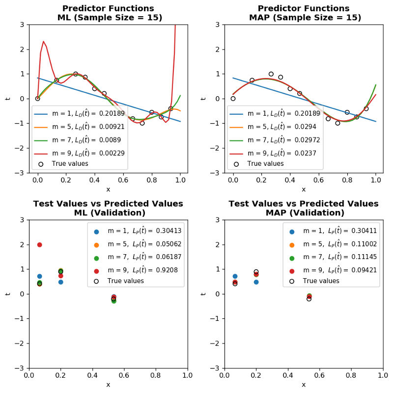
Observations:
-
lambdis the regularization constant and dictates how much our predictor \(\hat{t}\) fluctuates. Trylambd=10**-5andlambd=10**-1to see how it limits the function even for \(M=9\) -
Even for small sample size
N=15, MAP prevents overfitting of \(M=9\) -
When sample size
N=600and more, ML and MAP start to converge to the same results.
%matplotlib inline

import math
import numpy as np
import pandas as pd
import matplotlib.pyplot as plt
from scipy import stats, linalg


N = 15  # sample size
M = 9  # model order
domain_range = 1  # range of x values
lambd = 10**-3 # regularization constant

def t_true(x):
    return np.sin(2 * np.pi * x)


def fi(x, M):
    return np.array([x**i for i in range(0, M + 1)])


def data_generator(N, test_ratio=0.3):
    np.random.seed(42)  # To obtain the same result
    train_ratio = 1 - test_ratio
    limit_index = math.floor(N * train_ratio)
    nonoutlier_ratio = math.ceil(N * 0.7)

    X = np.linspace(0, domain_range, N, endpoint=False)
    nonoutlier_index = np.random.choice(X.shape[0], nonoutlier_ratio, replace=False)
    noise = np.array(stats.norm.rvs(loc=0, scale=0.35, size=N))
    noise[nonoutlier_index] = 0
    t = t_true(X) + noise

    # Randomization of dataset
    index = np.random.choice(X.shape[0], X.shape[0], replace=False)
    X = X[index]
    t = t[index]

    X_test = X[limit_index: None]
    X_train = X[: limit_index]

    t_test = t[limit_index: None]
    t_train = t[: limit_index]

    print(f" Training size: {X_train.shape[0]} and test size: {X_test.shape[0]}")

    return X_train, t_train, X_test, t_test


def design_matrix(X, m):
    Xd = np.array([fi(x, m) for x in X])
    return Xd


def fit_map(X, t, m):
    Xd = design_matrix(X, m)
    Xpenrose = np.matmul(linalg.inv(lambd * np.identity(m + 1) + np.matmul(Xd.T, Xd)), Xd.T)
    w = np.matmul(Xpenrose, t)
    return w

def fit_ml(X, t, m):
    Xd = design_matrix(X, m)
    Xpenrose = np.matmul(linalg.inv(np.matmul(Xd.T, Xd)), Xd.T)
    w = np.matmul(Xpenrose, t)
    return w

def predic(w, X_test, m):
    Xd = design_matrix(X_test, m)
    t_predic = np.matmul(Xd, w)
    return t_predic


def rms_calculator(t1, t2):
    """ L_P(t): Generalization loss"""

    result = np.sqrt(np.sum((t1 - t2)**2) / len(t1))
    result = round(result, 5)
    return result


def training_loss(t1, t2):
    """ L_D(t): Training loss"""
    result = np.sum((t1 - t2)**2) / len(t1)
    result = round(result, 5)
    return result


X_train, t_train, X_test, t_test = data_generator(N, test_ratio=0.2)

fig, ((ax1, ax2), (ax3, ax4)) = plt.subplots(nrows=2, ncols=2, figsize=(8, 8), dpi=120)

for m in [1, 5, 7, 9]:

    w = fit_ml(X_train, t_train, m)
    t_predic = predic(w, X_test, m)
    RMS = rms_calculator(t_test, t_predic)
    L_dt = training_loss(t_train, predic(w, X_train, m))

    x = np.linspace(0, domain_range, 50)
    y = predic(w, x, m)

    ax1.plot(x, y, label=f"m = {m}, " + r"$$L_{D}(\hat{t}) = $$" + f" {L_dt}")
    ax3.scatter(X_test, t_predic, label=f"m = {m}, " + r" $$L_{P}(\hat{t}) = $$" + f" {RMS}")


    w = fit_map(X_train, t_train, m)
    t_predic = predic(w, X_test, m)
    RMS = rms_calculator(t_test, t_predic)
    L_dt = training_loss(t_train, predic(w, X_train, m))

    x = np.linspace(0, domain_range, 50)
    y = predic(w, x, m)

    ax2.plot(x, y, label=f"m = {m}, " + r"$$L_{D}(\hat{t}) = $$" + f" {L_dt}")
    ax4.scatter(X_test, t_predic, label=f"m = {m}, " + r" $$L_{P}(\hat{t}) = $$" + f" {RMS}")


ax1.set_title(f"Predictor Functions\n ML (Sample Size = {N})", fontweight="bold")
ax1.set_ylim(-3, 3)
ax1.set_xlabel("x")
ax1.set_ylabel("t")
ax1.scatter(X_train, t_train, label=f"True values", marker="o", facecolor="none", edgecolor="k")
ax1.legend(fontsize=9)

ax3.set_title(f"Test Values vs Predicted Values\n ML (Validation)", fontweight="bold")
ax3.scatter(X_test, t_test, label="True values", marker="o", facecolor="none", edgecolor="k")
ax3.legend(fontsize=9)
ax3.set_xlabel("x")
ax3.set_ylabel("t")
ax3.set_xlim(0, 1)
ax3.set_ylim(-3, 3)

ax2.set_title(f"Predictor Functions\n MAP (Sample Size = {N})", fontweight="bold")
ax2.set_ylim(-3, 3)
ax2.set_xlabel("x")
ax2.set_ylabel("t")
ax2.scatter(X_train, t_train, label=f"True values", marker="o", facecolor="none", edgecolor="k")
ax2.legend(fontsize=9)

ax4.set_title(f"Test Values vs Predicted Values\n MAP (Validation)", fontweight="bold")
ax4.scatter(X_test, t_test, label="True values", marker="o", facecolor="none", edgecolor="k")
ax4.legend(fontsize=9)
ax4.set_xlim(0, 1)
ax4.set_ylim(-3, 3)
ax4.set_xlabel("x")
ax4.set_ylabel("t")
plt.tight_layout()
plt.savefig('map_results_1.png')
plt.show()
Training size: 12 and test size: 3
 |
| Previous post: Chapter 2: Part I | Next post: Chapter 2: Part III |