2. A “Gentle” Introduction Through Linear Regression
- 2.4 Bayesian framework:

2. A “Gentle” Introduction Through Linear Regression

2.4 Bayesian framework:

In frequentist framework, there are 2 distributions: true distribution approximated by empirical distribution and model distribution. However, in bayesian framework:

All data points are jointly distributed
Model parameters are also jointly distributed

At the end, bayesian framework considers all \(\theta\) values weighted with respect to data dependent belief. In short, everything is a random variable.

As a result, we have \(P(t_{D},w,t \vert X_{D}, x)\) as a posterior distribution. Given data set and a new point \((\mathcal{D},x)\), \(P(t \vert t_{D}, X_{D}, x) = P(t \vert \mathcal{D},x)\) is found using marginalization of \(P(t, w, t_{D} \vert X_{D}, x)\).

Using posterior \(P(t \vert \mathcal{D},x)\), predictor can be evaluated \(\hat{t}\). In a true bayesian framework, we have the explicit formula of the distribution function. By ignoring the domain points, we have

\[P(t, w, t_{D}) = \underset{\text{prior}}{P(w)} ~~ \underset{\text{likelihood}}{P(t_{D}~ \vert w)} ~~~ \underset{\text{distribution of new data}}{P(t \vert x)}\]

As a clarification, this equation holds due to the conditional independence of \({\rm t} ~ \vert {\rm w}\) and \({\rm t_{D}} ~ \vert {\rm w}\) as shown in the Figure 2.7 (book). In words, knowing only parameter w and \(t_{D}\) doesn’t give information about \(t\).

As mentioned our main purpose it to find \(P(t \vert \mathcal{D},x)\) and again dropping data points, we have

\[P(t \vert T_{D}) = \frac{P(t, T_{D})}{P(T_{D})} = \underset{\text{marginalization}}{\frac{\int P(t,w, T_{D})dw}{P(T_{D})}} = \frac{\int P(t, T_{D} \vert w) P(w) dw }{P(T_{D})}\] \[P(t \vert T_{D}) = \int P(t \vert w) ~ \left( \underset{\text{Bayes' rule}}{ \frac{P(T_{D} \vert w) P(w) }{P(T_{D})}} ~ \right) dw = \int P(t \vert w) P(w \vert T_{D}) dw\]

Finally reintroducing the data points, we obtain the key equation which is bayes prediction function

\[P(t \vert T_{D},x ) = \int P(t \vert x, w) P(w \vert \mathcal{D}) dw\]

Computing the posterior \(P(w \vert \mathcal{D})\) and predictive distribution \(P(t \vert x, w)\) is a difficult task. Especially in higher dimensions integrating out the model parameters becomes easily intractable. Using Gaussian prior \(\mathcal{N}(w \vert 0, \alpha^{-1})\), distribution of new data \(\mathcal{N}(t \vert \mathcal{M}(x,w), \beta^{-1})\) and likelihood \(\prod_{n=1}^{N} \mathcal{N}(t_{n} \vert \mathcal{M}(x,w), \beta^{-1})\), we can find predictive function distribution as

\[{\rm t} \vert {\rm x} \sim \mathcal{N}(t \vert \mathcal{M}(x,w_{MAP}~), S^{2}(x)) ~~~~ (2.36)\]

In this equation, \(S^{2}(x) = \beta^{-1} [ 1 + \phi(x)^{T} ( \lambda I + X_{D}^{T} X_{D})^{-1} \phi(x)]\). However, deriving this equation is an extremely tedious task which also fortifies the claim about the difficulty of integration process. A detailed step by step derivation can be found in mathematicalmonk’s videos here (watching him struggle might also produce a confidence boost).

ML and MAP vs bayesian

Comparing the returned distribution of each approach, it is easy to see distinction

ML: \(\mathcal{N}(t \vert \mathcal{M}(x,w_{ML}~), \beta^{-1}(x))\)
MAP: \(\mathcal{N}(t \vert \mathcal{M}(x,w_{MAP}~), \beta^{-1}(x))\)
Bayesian: \(\mathcal{N}(t \vert \mathcal{M}(x,w_{MAP}~), S^{2}(x))\), variance changes with w.r.t. x

In bayesian approach, variance changes with given new data point. In addition, as \(N \to \infty, S^{2}(x) \to 1 / \beta\)

Bayesian `code practice`

N is the sample size
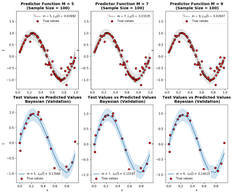
\(\mathcal{L}_{D}~(\hat{t})\) is training loss
\(\mathcal{L}_{P}~(\hat{t})\) is generalization loss which is approximated by validation using Root Mean Squared Metric
\(\lambda\) is regularization constant

Observations:

lambd is the regularization constant and dictates how much our predictor \(\hat{t}\) fluctuates. Try lambd=10**-5 and lambd=10**-1 to see how it limits the function even for \(M=9\)
Even for small sample size N=15, MAP prevents overfitting of \(M=9\)
When sample size N=600 and more, ML and MAP start to converge to the same results.

%matplotlib inline

import math
import numpy as np
import pandas as pd
import matplotlib.pyplot as plt
from scipy import stats, linalg


N = 100  # sample size
M = 9  # model order
domain_range = 1  # range of x values
alpha = 10**-2
beta = 10


def t_true(x):
    return np.sin(2 * np.pi * x)


def fi(x, M):
    return np.array([x**i for i in range(0, M + 1)])


def data_generator(N, test_ratio=0.3):
    np.random.seed(42)  # To obtain the same result
    train_ratio = 1 - test_ratio
    limit_index = math.floor(N * train_ratio)
    nonoutlier_ratio = math.ceil(N * 0.7)

    X = np.linspace(0, domain_range, N, endpoint=False)
    nonoutlier_index = np.random.choice(X.shape[0], nonoutlier_ratio, replace=False)
    noise = np.array(stats.norm.rvs(loc=0, scale=0.35, size=N))
    noise[nonoutlier_index] = 0
    t = t_true(X) + noise

    # Randomization of dataset
    index = np.random.choice(X.shape[0], X.shape[0], replace=False)
    X = X[index]
    t = t[index]

    X_test = X[limit_index: None]
    X_train = X[: limit_index]

    t_test = t[limit_index: None]
    t_train = t[: limit_index]

    print(f" Training size: {X_train.shape[0]} and test size: {X_test.shape[0]}")

    return X_train, t_train, X_test, t_test


def design_matrix(X, m):
    Xd = np.array([fi(x, m) for x in X])
    return Xd


def predic_bayesian(X_train,t_train,m,x):

    Xd = design_matrix(X_train, m)
    Fd = design_matrix(x, m)
    A = linalg.inv((alpha/beta) * np.identity(m + 1) + np.matmul(Xd.T, Xd))
    Xpenrose = np.matmul(A, Xd.T)
    w = np.matmul(Xpenrose, t_train)
    t_predic = np.matmul(Fd, w)

    t_variance = beta**-1 * (1 + np.diagonal(np.matmul(np.matmul(Fd,A) ,Fd.T )))
    return t_predic, t_variance


def rms_calculator(t1, t2):
    """ L_P(t): Generalization loss"""

    result = np.sqrt(np.sum((t1 - t2)**2) / len(t1))
    result = round(result, 5)
    return result


def training_loss(t1, t2):
    """ L_D(t): Training loss"""
    result = np.sum((t1 - t2)**2) / len(t1)
    result = round(result, 5)
    return result


X_train, t_train, X_test, t_test = data_generator(N, test_ratio=0.2)

# print(X_train, t_train, X_test, t_test)

fig, ax = plt.subplots(nrows=2, ncols=3, figsize=(12, 10), dpi=120)
print(ax.shape)
count = 0
for m in [5, 7, 9]:

    ### Bayesian learning
    t_predic, t_variance = predic_bayesian(X_train,t_train,m,X_test)

    t_predic_train, t_variance_train = predic_bayesian(X_train,t_train,m,X_train)

    L_dt = training_loss(t_train, t_predic_train)
    RMS = rms_calculator(t_test, t_predic)

    order = np.argsort(X_train)

    ax[0][count].plot(X_train[order], t_predic_train[order],\
             '-', color='gray', label=f"m = {m}, " + r"$$L_{D}(\hat{t}) = $$" + f" {L_dt}")
    ax[0][count].fill_between(X_train[order], t_predic_train[order] - 2*t_variance_train[order], \
                     t_predic_train[order] + 2*t_variance_train[order], color='gray', alpha=0.2)

    ax[0][count].set_title(f"Predictor Function M = {m}\n (Sample Size = {N})", fontweight="bold")
    ax[0][count].set_xlabel("x")
    ax[0][count].set_ylabel("t")

    order = np.argsort(X_train)
    ax[0][count].scatter(X_train[order], t_train[order], label=f"True values", marker="o", facecolor="r", edgecolor="k")
    ax[0][count].legend(fontsize=9)


    order = np.argsort(X_test)
    ax[1][count].plot(X_test[order], t_predic[order], '-', label=f"m = {m}, " + r" $$L_{P}(\hat{t}) = $$" + f" {RMS}")
    ax[1][count].fill_between(X_test[order], t_predic[order] - 2*t_variance[order], \
                     t_predic[order] + 2*t_variance[order], alpha=0.2)


    order = np.argsort(X_test)
    ax[1][count].set_title(f"Test Values vs Predicted Values\n Bayesian (Validation)", fontweight="bold")
    ax[1][count].scatter(X_test[order], t_test[order], label=f"True values", marker="o", facecolor="r", edgecolor="k")
    ax[1][count].legend(fontsize=9)
    ax[1][count].set_xlabel("x")
    ax[1][count].set_ylabel("t")


    count += 1


# plt.savefig('map_results_1.png')
plt.show()

Marginal likelihood

Following formula is named marginal log likelihood

\[P(t_{D}~ \vert X_{D}) = \int P(w) \prod_{n=1}{N} P(t_{n}~ \vert x_{n},w) dw\]

and this approach enables model selection without validation by including prior information to likelihood process. Calculating the marginal likelihood of running example:

\[P(t_{D}~ \vert X_{D}) \sim \mathcal{N}(0, \alpha^{-1} X_{D}~X_{D}^{T} + \beta^{-1} I )\]

Since normalization constant of a Gaussian distribution depends on variance which \(\alpha^{-1} X_{D}~X_{D}^{T} + \beta^{-1} I\), peak value of \(P(t_{D}~ \vert X_{D})\) changes with \(\alpha\) and \(\beta\) parameters.

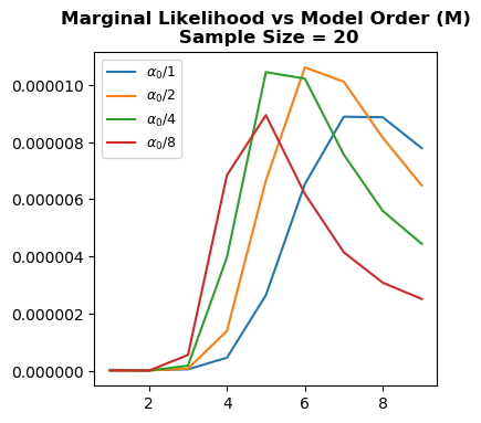
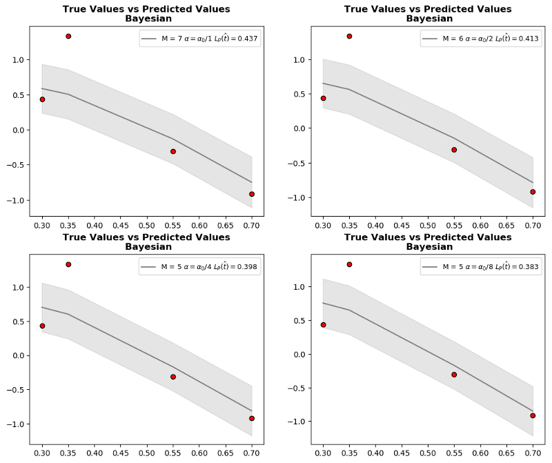
Let’s go through the whole process. At first, we choose \(\alpha, \beta\) and calculate marginal log likelihood \(P(t_{D}~ \vert X_{D})\) and choose the \(M\) yielding peak value. However, if we graph \(P(t_{D}~ \vert X_{D})\) vs. \(M\) with different \(\alpha\) values, it is clear that even though peak \(M\) values are similar we cannot exactly pin down the optimum value with only checking a single \(\alpha\). In short, we again have a hyperparameter to tune. As we mentioned earlier, changing \(\alpha\) affects variance \(alpha^{-1} X_{D}~X_{D}^{T} + \beta^{-1} I\) which changes normalization and consequently peak value of \(P(t_{D}~ \vert X_{D})\).

Finally, assigning priors to \(\alpha\) and \(M\) also leads to hierarchical models that will be covered in post 7.

Marginal likelihood `code practice`

\(\mathcal{L}_{P}~(\hat{t})\) is generalization loss which is approximated by validation using Root Mean Squared Metric
\(\alpha\) is precision for w
\(\beta\) is precision for data points